Uproot framework
This is an analysis code in uproot that can be used to analyse the 13 TeV open data.
Get the Code
You can access the code at the link below:
The framework consists of 5 main files:
- the Analysis files perform the particular object selection;
- the Plotting files make Data / Prediction plots from saved results;
- the Samples files specify the particular samples to use;
- the Cuts files specify the particular cuts to implement;
- the Histograms files specify which plots to make.
Read about these analyses in the Example Analyses with the 13 TeV Data for Education section
Get theData
The 13 TeV ATLAS Open Data are hosted on the CERN Open Data portal. The framework can access the samples in two ways:
- reading them online directly.
- reading them form a local storage (the samples need to be downloaded locally).
First Time Setup
This framework uses:
It does not have any dependency on ROOT.
To install the dependencies run the following code:
python3 -m pip install -U numpy pandas uproot matplotlib lmfit tables --user
You only have to do this once.
Running an Analysis
The files in the root directory of the installation are the various analysis codes.
You can run a preconfigured analysis via
python3 HZZAnalysis.py
The first portion of an analysis code specifies the packages that need to be imported:
import uproot    		     	(to read .root files)

import pandas as pd			(for dataframe to hold the data)

import time				(to time the code)

import math				(for mathematical functions such as trig)

import numpy as np			(for numeric calculations)

import matplotlib.pyplot as plt	(to make plots)
The second portion of an analysis code specifies information such as the locations of files:
tuple_path = "https://atlas-opendata.web.cern.ch/atlas-opendata/samples/2020/4lep/"	(file location)

stack_order = [r'$Z,t\bar{t}$','ZZ']					(order of coloured bars)
XSamples.py contains the individual files that are to be used for the different processes:
samples = {

    'data': {
        'list' : ['data_A','data_B','data_C','data_D']
    },
 ...
}
The names chosen for the processes are important as they are the keys that are used later in the infofile.py to determine the necessary scaling factors for correct plotting.
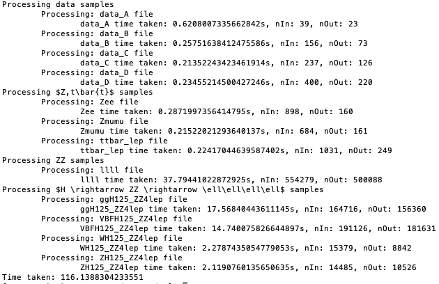
Execution times are ~ 200 seconds.
Plotting the Results
The resulting plots will be saved in the root directory.
The plot_data function enables the user to steer the plotting process. Each analysis has its own plot_data function to accomodate changes in histograms that the user may want to plot.
General information for plotting include the x axis located in the XHistograms.py files:
'bin_width':5,
'num_bins':34,
'xrange_min':80,
'log_y':False,
The names of the histograms to be drawn can be specified like so:
mllll = {
...
}

hist_dict = {'mllll':mllll}
Definiton of plot content
Each plot consists of several aspects, which may include data and errors. A definition of plot content may look like this:
data_x,_ = np.histogram(data['data'][x_variable].values/1000, bins=bins)
data_x_errors = np.sqrt(data_x)

signal_x = None
if signal_format=='line':
    signal_x,_ = np.histogram(data[signal][x_variable].values/1000,bins=bins,weights=data[signal].totalWeight.values)
elif signal_format=='hist':
    signal_x = data[signal][x_variable].values/1000
    signal_weights = data[signal].totalWeight.values
    signal_color = HZZSamples.samples[signal]['color']

mc_x = []
mc_weights = []
mc_colors = []
mc_labels = []
mc_x_tot = np.zeros(len(bin_centres))

for s in stack_order:
    mc_labels.append(s)
    mc_x.append(data[s][x_variable].values/1000)
    mc_colors.append(HZZSamples.samples[s]['color'])
    mc_weights.append(data[s].totalWeight.values)
    mc_x_heights,_ = np.histogram(data[s][x_variable].values/1000,bins=bins,weights=data[s].totalWeight.values)
    mc_x_tot = np.add(mc_x_tot, mc_x_heights)

mc_x_err = np.sqrt(mc_x_tot)
A stack shows the different processes specified in "stack_order" stacked upon each other to give an idea of the composition of the simulated data. The definitions for these individual processes are defined under XSamples.py. Each process has a certain colour and a list of contributing parts that comprise it. These contributing parts are the keys used in both the run configuration and the infofile.py.
data is geared toward the standard representation of data. Since the data does not need to be scaled there is no need to align the used names in contributions with those found in the infofile.py.
The defined plots can the be drawn like so:
plt.axes([0.1,0.3,0.85,0.65]) #(left, bottom, width, height)
main_axes = plt.gca()
main_axes.errorbar( x=bin_centres, y=data_x, yerr=data_x_errors, fmt='ko', label='Data')
mc_heights = main_axes.hist(mc_x,bins=bins,weights=mc_weights,stacked=True,color=mc_colors, label=mc_labels)
if Total_SM_label:
    totalSM_handle, = main_axes.step(bins,np.insert(mc_x_tot,0,mc_x_tot[0]),color='black')
if signal_format=='line':
    main_axes.step(bins,np.insert(signal_x,0,signal_x[0]),color=HZZSamples.samples[signal]['color'], linestyle='--',
                label=signal)
elif signal_format=='hist':
    main_axes.hist(signal_x,bins=bins,bottom=mc_x_tot,weights=signal_weights,color=signal_color,label=signal)
main_axes.bar(bin_centres,2*mc_x_err,bottom=mc_x_tot-mc_x_err,alpha=0.5,color='none',hatch="////",
            width=h_bin_width, label='Stat. Unc.')

main_axes.set_xlim(left=h_xrange_min,right=bins[-1])
main_axes.xaxis.set_minor_locator(AutoMinorLocator()) # separation of x axis minor ticks
main_axes.tick_params(which='both',direction='in',top=True,labeltop=False,labelbottom=False,right=True,labelright=False)
main_axes.set_ylabel(r'Events / '+str(h_bin_width)+r' GeV',fontname='sans-serif',horizontalalignment='right',y=1.0,fontsize=11)
if h_log_y:
    main_axes.set_yscale('log')
    smallest_contribution = mc_heights[0][0]
    smallest_contribution.sort()
    bottom = smallest_contribution[-2]
    top = np.amax(data_x)*h_log_top_margin
    main_axes.set_ylim(bottom=bottom,top=top)
    main_axes.yaxis.set_major_formatter(CustomTicker())
    locmin = LogLocator(base=10.0,subs=(0.1,0.2,0.3,0.4,0.5,0.6,0.7,0.8,0.9),numticks=12)
    main_axes.yaxis.set_minor_locator(locmin)
else:
    main_axes.set_ylim(bottom=0,top=(np.amax(data_x)+math.sqrt(np.amax(data_x)))*h_linear_top_margin)
    main_axes.yaxis.set_minor_locator(AutoMinorLocator())

plt.text(0.05,0.97,'ATLAS',ha="left",va="top",family='sans-serif',transform=main_axes.transAxes,style='italic',weight='bold',fontsize=13)
plt.text(0.19,0.97,'Open Data',ha="left",va="top",family='sans-serif',transform=main_axes.transAxes,fontsize=13)
plt.text(0.05,0.9,'for education only',ha="left",va="top",family='sans-serif',transform=main_axes.transAxes,style='italic',fontsize=8)
plt.text(0.05,0.86,r'$\sqrt{s}=13\,\mathrm{TeV},\;\int L\,dt=$'+lumi_used+'$\,\mathrm{fb}^{-1}$',ha="left",va="top",family='sans-serif',transform=main_axes.transAxes)
plt.text(0.05,0.78,plot_label,ha="left",va="top",family='sans-serif',transform=main_axes.transAxes)

# Create new legend handles but use the colors from the existing ones
handles, labels = main_axes.get_legend_handles_labels()
if signal_format=='line':
    handles[labels.index(signal)] = Line2D([], [], c=HZZSamples.samples[signal]['color'], linestyle='dashed')
if Total_SM_label:
    uncertainty_handle = mpatches.Patch(facecolor='none',hatch='////')
    handles.append((totalSM_handle,uncertainty_handle))
    labels.append('Total SM')

# specify order within legend
new_handles = [handles[labels.index('Data')]]
new_labels = ['Data']
for s in reversed(stack_order):
    new_handles.append(handles[labels.index(s)])
    new_labels.append(s)
if Total_SM_label:
    new_handles.append(handles[labels.index('Total SM')])
    new_labels.append('Total SM')
else:
    new_handles.append(handles[labels.index('Stat. Unc.')])
    new_labels.append('Stat. Unc.')
if signal is not None:
    new_handles.append(handles[labels.index(signal)])
    new_labels.append(signal_label)
main_axes.legend(handles=new_handles, labels=new_labels, frameon=False, loc=h_legend_loc)
The order of the stack is determined by "stack_order".
If everything was successful, the code will show output similar to below.
In Depth Information
Analysis Code
The analysis codes are located in the root folder. They are used to make plots.
It is recommended to start out by modifying one of the existing analyses, e.g. the HZZAnalysis located in HZZAnalysis.py.