C++ framework
The framework is built using the C++ language and interfaces with the ROOT framework.
Get the code
You can access the source code on GitHub:
The framework consists of two main parts:
- the analysis, located within the "Analysis" directory: it performs the particular object selection and stores the output histograms;
- the plotting, located within the "Plotting" directory: it makes the final Data / Prediction plots.
Read about all the available analyses in the Example Analyses with the 13 TeV Data for Education section
Get the data
The 13 TeV ATLAS Open Data are hosted on the CERN Open Data portal. The framework can access the samples in two ways:
- reading them online directly (be default, they are stored in a GitHub repository);
- reading them form a local storage (the samples need to be downloaded locally).
First time set up
Before you start using the framework, ensure you have the following installed:
- ROOT Framework: Essential for the framework's operation. Go to ROOT documentation and follow the instructions to set it up.
- GCC Compiler: Required to compile the source code. The framework was compiled using gcc v6.20.
The framework is tested and compatible with:
- GCC Version: 6.20
- ROOT Version: 6.10.04
The analyses
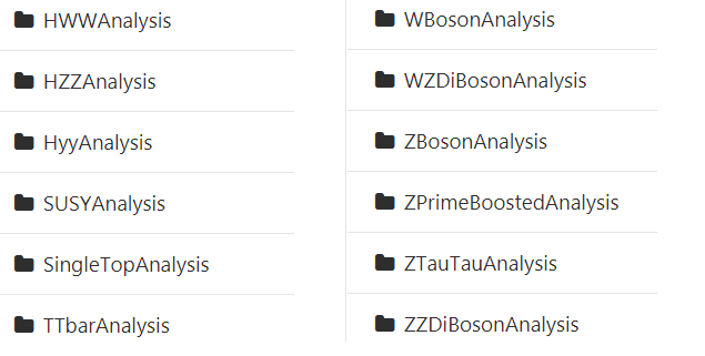
The analysis code is located in the Analysis folder, with 12 sub-folders corresponding to the 12 examples of physics analysis documented in Physics analysis examples. The naming of the sub-folders follows a simple rule: "NNAnalysis", where NN can be WBoson, ZBoson, TTbar, SingleTop, WZDiBoson, ZZDiBoson, HZZ, HWW, Hyy, ZPrimeBoosted, ZTauTau and SUSY.

Each analysis sub-folder contains the following files:
- analysis main code (NNAnalysis.C): it makes all the selection and stores the output histograms;
- analysis main header (NNAnalysis.h): it defines the histograms and gives access to the variables stored in the input samples;
- histogram header (NNAnalysisHistograms.h): it defines the name of output histograms;
- analysis main-control code (main_NNAnalysis.C): it controls which input samples are going to be used and their location;
- a bash script (run.sh), executed via a Linux/UNIX shell called source: helps you in running the analysis interactively.
- in case you used the welcome script, the output directory (Output_NNAnalysis) will be created: this is the place where the output of the analysis code (one file with histograms per each input sample) will be stored. Warning: if the output directory does not exist, the code will fail, please create always an empty one!
As an example, in the case of the HWWAnalysis, the sub-folder looks like this (Output_HWWAnalysis was not created yet):
Run an analysis
In the main directory, do the first setup of the code by typing in the terminal:
./welcome.sh
or in case you have installed the source shell:
source welcome.sh
This will ask you if you want to create automatically all the output directories in all the 12 analysis sub-folders, or to erase their contents in case it is needed.
After this, change to any of the analysis sub-folders and open using your preferred text-editor the analysis main-control code (main_NNAnalysis.C): it controls the location of the input samples, please find the line:
// path to your local directory *or* URL, please change the default one!
TString path = "";
and adapt it properly to your specific case.
After that, execute the code via the command line using:
./run.sh
or
source run.sh
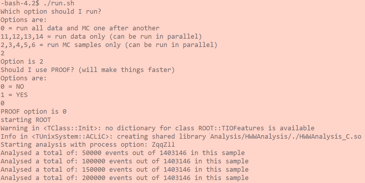
The script will interactively ask you for two options which you can type directly (0, 1,..) in the terminal and hit "ENTER":
- The first option will ask you: do you want to run over all the samples one-by-one, or to run over only data or only simulated samples? The latter options can help you to speed up the analysis, as you can run several samples in several terminals.
- The second option will ask you: do you want to use the Parallel ROOT Facility (PROOF), a ROOT-integrated tool that enables the analysis of the input samples in parallel on a many-core machine? If your ROOT version has PROOF integrated, it will speed up the analysis by a factor of roughly 5.
After you choose the options, the code will compile and create the needed ROOT shared libraries, and the analysis selection will begin: it will run over each input sample defined in main_NNAnalysis.C.
If everything was successful, the code will create in the output directory (Output_NNAnalysis) a new file with the name of the corresponding sample (data, ttbar,...).

To clean all shared and linked libraries after running, you can use a script called clean.sh located in the main directory.
The plots
The plotting code is located in the Plotting folder and contains the following files:
- plotting main code (Plotting.cxx): it makes all plot magic and controls automatically what to do for each of the 12 analyses;
- plotting main header (Plotting.h): it defines all the needed bits and pieces for the plotting code;
- helper directory (list_histos): inside it you will find 12 control files with names HistoList_ANALYSISNAME.txt, each of these controls which histograms are going to be used and plotted for each analysis;
- helper directory (inputfiles): inside it you will find 12 control files with names Files_ANALYSISNAME.txt, each of these controls which input samples exactly are going to be used for this particular analysis, their cross-section and sum of weights. DO NOT CHANGE!!!
- bash script (plotme.sh): helps you in running the plotting code interactively, please use it!
- a makefile (Makefile): a set of directives used by a make build automation tool to generate the output executable;
- in case you used the welcome script, the output directory (histograms): it will contain the output plots! Do not forget to rename it in case you run over several analyses!
Plotting the Results
In the main Plotting directory, execute in the terminal:
./plotme.sh
or in case you have installed the source shell:
source plotme.sh
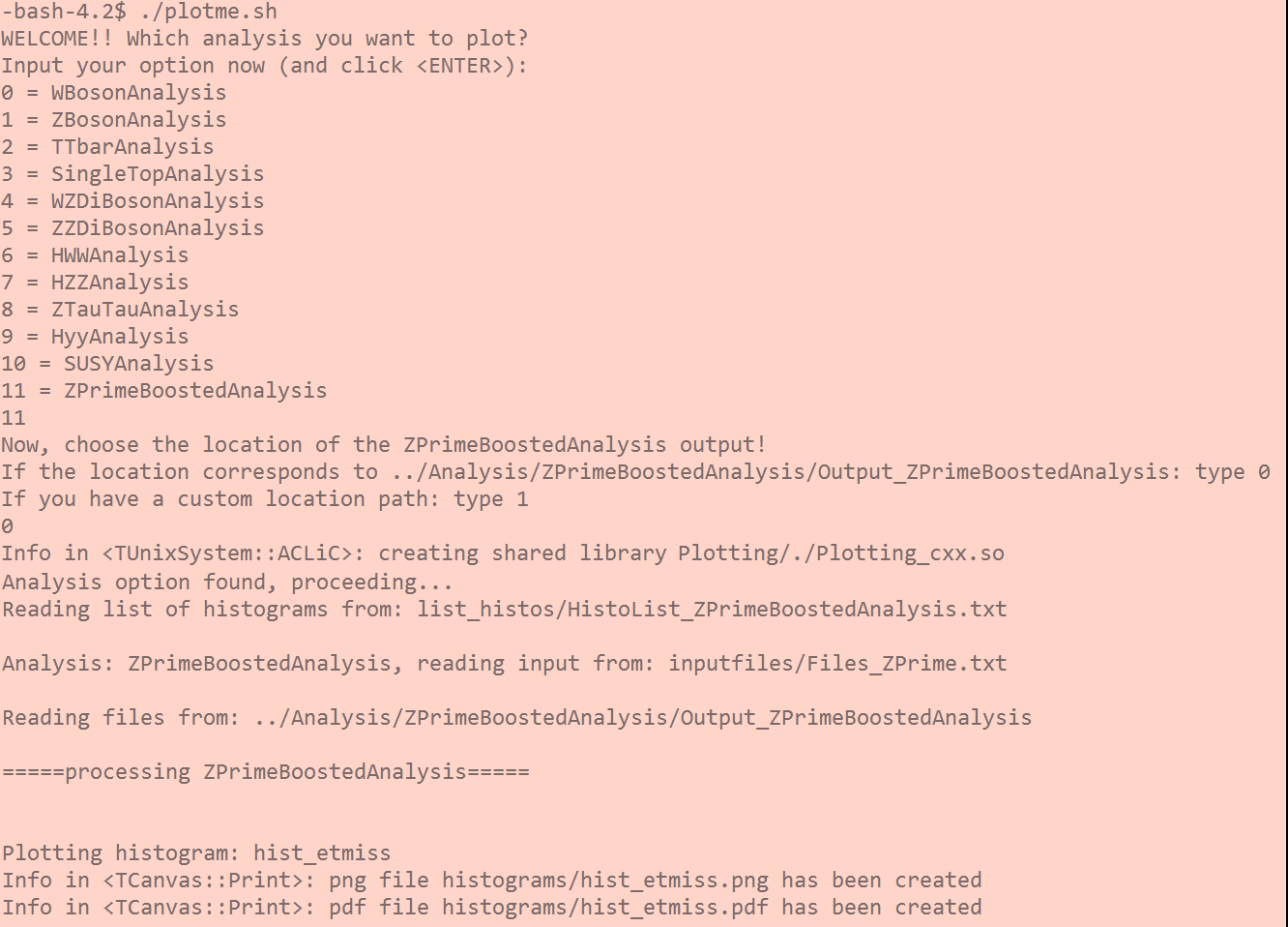
The script will interactively ask you for two options which you can type directly (0, 1,..) in the terminal and hit "ENTER":
- The first option will be: which analysis exactly out of the 12 you want to plot?
- The second option will ask you for the location of the Output_NNAnalysis directory that was created by running the Analysis code.
After you choose the options, the code will compile and create the needed ROOT shared libraries, and the plotting will begin. If everything was successful, the code will create in the output directory (histograms) the corresponding plots defined in HistoList_ANALYSISNAME.txt.

To clean all shared and linked libraries after running, you can use a script called clean.sh located in the main directory.
Additional information about the plotting code:
-
In case you want to see the data and MC event yields: change "#define YIELDS 0" to "#define YIELDS 1" in Plotting.cxx and remake the plots;
-
In case you want to add the normalised signal to the plots: change "#define NORMSIG 0" to "#define NORMSIG 1" in Plotting.cxx and remake the plots;
-
In case something is not working: by changing "#define DEBUG 0" to "#define DEBUG 1" in Plotting.cxx, a lot of debug information will appear, this can help you trace the origin of any possible problem (usually, these could be: the directory histograms does not exist, a wrong path for the location of the input files is given, a wrong or non-existent histogram name is requested, one or several input files from the analysis are missing or failed,..)
-
In case you want to compile the code instead of the using the plotme script, type "make clean; make" and then run the code with ./plot [NNAnalysis] [location of Output_NNAnalysis]
How to add a new variable in the analysis code and plot it
To add a new variable called new_variable (which, as an example, will contain the information of something), save it as a new histogram called h_new and make a plot of it, follow the instructions below:
(1) Add in the header (NNAnalysis.h) the new histogram (in the function public TSelector where you see the definitions of other histograms):
TH1F *h_new = 0;
(2) Add in the histogram header (NNAnalysisHistograms.h) four new lines:
inside the function define_histograms() add:
h_new = new TH1F("h_new", "Description of the new variable; X axis name ; Y axis name ", number of bins , minimum bin value , maximum bin value);
inside the function FillOutputList() add:
GetOutputList()->Add(h_new);
inside the function WriteHistograms() add:
h_new->Write();
inside the function FillHistogramsGlobal() add:
if (s.Contains("h_new")) h_new->Fill(m,w);
(3) And finally, inside the main analysis code NNAnalysis.C you need to define a new variable (in this case an integer called new_variable), connect it to the value of the branch something that exists in the input samples (those are listed in the analysis header NNAnalysis.h after "Declaration of leaf types") and save the newly created histogram inside the function Process after the line that reads the content of the TTree (fChain->GetTree()->GetEntries()>0)
int new_variable = something;

FillHistogramsGlobal( new_variable, weight, "h_new");
where the weight is the multiplication of scale factors and Monte Carlo weight.
(4) Now run the analysis code as usual again over all the samples and check that the new histogram h_new appears in the produced output files.
(5) Analysis part is done, go to Plotting part and in the list_histos directory in HistoList_ANALYSISNAME.txt file add one new line:
h_new
(with no empty lines before or after it!).
(6) Execute the plotting code as usual (no need to change the code itself at all), and you will find the new histogram in histograms/h_new.png!