Calibrations

As particles travel through the detector material before reaching the electromagnetic calorimeter, they can lose energy through interactions such as bremsstrahlung for electrons and Compton scattering or pair production for photons. Additionally, not all the energy from the resulting electromagnetic showers is contained within the reconstructed cluster, as some can leak laterally or longitudinally, escaping the cluster boundaries or penetrating through the electromagnetic calorimeter. Calibrations are needed for accurate energy measurements of electrons and photons.

Calibration also corrects for the non-uniform and non-linear response of the electromagnetic calorimeter. Furthermore, raw signals include background noise, which must be subtracted to isolate the true signal.

By addressing these factors, calibration significantly improves the energy resolution and accuracy of particle identification, ensuring that the measured energies reflect the true energies of the particles.

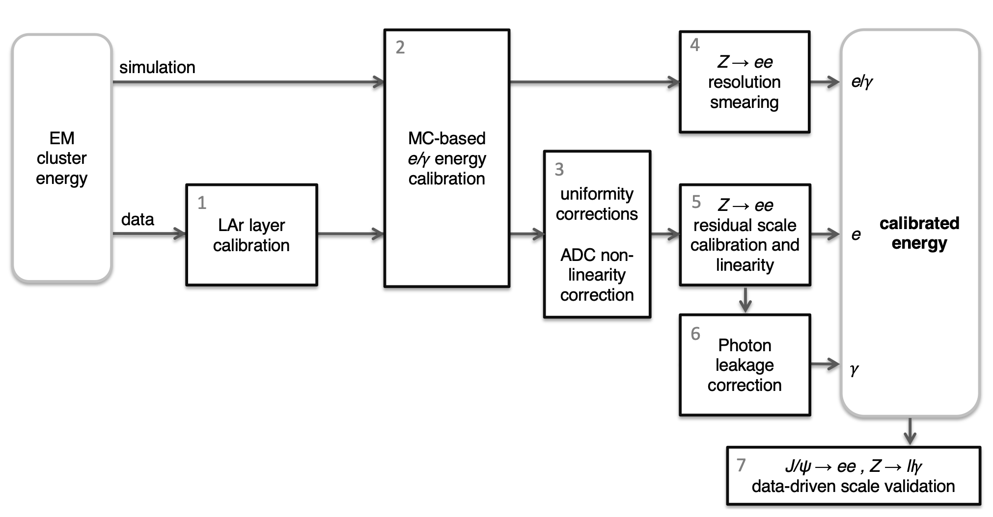
Below, you can find a schema of the calibration process for electrons and photons. The explanation of each step is shortly explained next.

Fig. 1: Schematic overview of the electron and photon energy calibration procedure in ATLAS.

Liquid Argon Layer Calibration

The electromagnetic calorimeter in the ATLAS detector is a sampling calorimeter that uses liquid argon (LAr) as the active medium. The electromagnetic calorimeter is divided into multiple layers, and the LAr layer calibration ensures that the energy deposited in each layer is accurately measured and corrected for any discrepancies. The primary purpose of LAr layer calibration is to account for variations in the detector response across different layers of the electromagnetic calorimeter. Each layer of the calorimeter has a different sensitivity and response to incoming particles, and these variations can affect the accuracy of the energy measurement.

The LAr layer calibration begins by measuring the detector response to known energy deposits. This is typically achieved using test beams where particles with well-defined energies are directed into the detector. The energy deposited in each layer of the electromagnetic calorimeter is recorded, providing baseline measurements for the calibration. Monte Carlo simulations are used to model the energy deposition in the calorimeter layers. These simulations consider the geometry and material properties of the detector, offering a representation of how particles interact with the detector. The simulated responses are then compared with the actual data obtained from collision events. The LAr layer calibration is a calibration on data only, ensuring that real detector performance is accounted for.

Calibration constants are obtained by comparing the simulated energy deposits with the measured energy deposits. These constants are used for correcting any discrepancies between the expected and observed responses. Each layer of the electromagnetic calorimeter has its specific calibration constants, to address its response characteristics.

Once these calibration constants are determined, they are applied to the data collected during actual physics runs. This involves adjusting the raw energy measurements from each layer to match the calibrated response. The corrected energy measurements from all layers are then summed to obtain the total calibrated energy for each particle.

Monte Carlo-Based Energy Calibration

This process begins with Monte Carlo simulations. These simulations take into account the geometry and material properties of the electromagnetic calorimeter, including electromagnetic showers, energy losses, and scattering effects. The simulated energy deposits are then compared with actual measurements obtained from controlled test beam experiments and real collision events to identify any discrepancies.

Based on these comparisons, calibration constants are derived to correct the observed discrepancies. These constants are calculated to adjust the raw energy measurements from the electromagnetic calorimeter, ensuring that the detector's response is uniform across the entire energy range and for different regions of the calorimeter.

Once the calibration constants are established, they are first applied to the Monte Carlo simulations, making sure that they reflect the expected performance of the detector. Once validated, these calibration constants are then applied to the actual experimental data, adjusting the raw energy measurements to agree with the calibrated simulations.

Uniformity Corrections

Uniformity corrections are done to achieve consistency in the energy measurements across the entire electromagnetic calorimeter. The electromagnetic calorimeter is composed by many individual cells, each of which can have slight variations in their response to incoming particles due to manufacturing differences, aging, or operational conditions. The goal of uniformity corrections is to adjust for these variations, so that a particle depositing the same amount of energy in different parts of the calorimeter produces the same signal. This correction tries to mantain an uniform response across the entire detector, which is necessary for energy measurements.

Uniformity corrections are typically derived using test beam data and in-situ calibration techniques. Test beams of particles with known energies are directed into various regions of the electromagnetic calorimeter to measure the response of each cell. These measurements are compared to the expected uniform response, and corrections are calculated to account for any deviations. In-situ calibration uses well-known physics processes, such as the invariant mass of particle decays, to further refine these corrections during actual data-taking periods. The derived corrections are then applied to the raw energy measurements to achieve uniformity across the calorimeter.

ADC Non-Linearity Corrections

Analog-to-Digital Converters (ADCs) are used in the electromagnetic calorimeter to digitize the analog signals generated by the particle interactions. Ideally, the ADC response should be linear, meaning that the output digital signal should be directly proportional to the input analog signal. However, in reality, ADCs can exhibit non-linear behavior, where the relationship between the input and output signals deviates from a straight line.

ADC non-linearity corrections are applied to get the digitized energy measurements to reflect the true energy deposited in the calorimeter. This corrections are determined through calibration processes where known signals are input to the ADC, and the output is measured. By comparing the actual output to the expected linear response, a correction function is derived that maps the non-linear ADC output back to the correct linear value. The corrections are applied to the digitized signals from the electromagnetic calorimeter to correct any non-linearities introduced by the ADCs.

Z -> ee Resolution Smearing

The primary purpose of resolution smearing is to account for the differences between the idealized detector response as modeled in Monte Carlo simulations and the actual performance of the detector. In real experimental conditions, various factors such as electronic noise, detector material imperfections, and other systematic uncertainties can degrade the energy resolution. Resolution smearing helps bridge this gap by adjusting the Monte Carlo simulations to better match the real data.

The process begins with the identification of $Z\rightarrow e^+ e^-$ events in both the experimental data and Monte Carlo simulations. The $Z$ boson decays into a pair of electrons, providing a clean and well-understood signal that can be used for calibration and resolution studies.

The energy resolution for the $Z\rightarrow e^+ e^-$ events is determined for both the data and the Monte Carlo simulations. This involves measuring the invariant mass distribution of the electron pairs. The invariant mass should peak at the mass of the $Z$ boson (approximately 91 GeV/c²), but due to resolution effects, this peak will be broader in real data.

By comparing the width of the invariant mass peak (resolution) in data and Monte Carlo simulations, smearing parameters are derived. These parameters quantify the additional broadening required to match the Monte Carlo resolution to the data resolution. The process involves fitting the invariant mass distributions and extracting the resolution differences.

The derived smearing parameters are then applied to the energy measurements in the Monte Carlo simulations. This is done by adding a Gaussian smearing term to the electron energies in the Monte Carlo events, effectively broadening the energy distribution to match the data. This smearing mimics the effects of the various factors that degrade resolution in the actual detector.

The smeared Monte Carlo simulations are then compared again to the real data to validate the smearing process. The invariant mass distributions of the $Z\rightarrow e^+ e^-$ events should now show better agreement between the data and the simulations, indicating that the resolution smearing has been successfully applied.

EXAMPLE PLOT HERE

Z -> ee Residual Scale Calibration and Linearity Correction

After initial calibrations, small discrepancies can remain due to various detector effects. The $Z\rightarrow e^+e^-$ process provides a well-defined and abundant source of electrons to calibrate further.

For the residual scale calibration, events where the Z boson decays into an electron-positron pair ($Z\rightarrow e^+ e^-$) are selected from the data. These events are chosen because the invariant mass of the electron-positron pair should peak sharply at the known mass of the Z boson (approximately 91 GeV/c²). The invariant mass of the electron-positron pairs is then calculated for the selected events. This distribution is then compared to the expected peak at the Z boson mass. Discrepancies between the measured peak position and the known Z boson mass indicate a need for scale correction.

Correction factors are derived to adjust the energy scale so that the peak of the invariant mass distribution aligns precisely with the Z boson mass. These factors are applied to the data to correct any remaining biases in the energy scale.The corrected energy measurements are validated by re-evaluating the invariant mass distribution of the $Z\rightarrow e^+ e^-$ events. A well-calibrated detector will show the peak at the Z boson mass with minimal residual discrepancies.

Then, the linearity calibration ensures that the detector’s response is proportional across a wide range of energies. A linear response means that the ratio of the measured energy to the true energy remains constant, regardless of the energy of the incoming particle.

The $Z \rightarrow e^+e^-$ process provides electrons with a broad range of energies. By analyzing these electrons, we can assess the detector’s linearity across this energy spectrum. The invariant mass of electron-positron pairs is examined in different energy bins. Each bin represents a range of electron energies, allowing for a detailed assessment of the detector’s response at various energy levels. For each energy bin, the invariant mass peak of the electron-positron pairs is analyzed. If the detector response is linear, the measured invariant mass should consistently peak at the Z boson mass, regardless of the energy bin. If deviations from linearity are observed, correction factors are derived to adjust the energy measurements. These factors ensure that the detector’s response is linear, meaning that any electron, regardless of its energy, is measured accurately.

EXAMPLE PLOT HERE

Photon Leakage Correction

The photon leakage correction addresses the issue of energy leakage, where some of the energy deposited by photons is not fully contained within the electromagnetic calorimeter.

The primary goal of photon leakage correction is to make sure that the energy measured for photons in the electromagnetic calorimeter accurately reflects their true energy. Photon-induced showers in the electromagnetic calorimeter can extend beyond the boundaries of the reconstructed cluster. This extension can be lateral, where the energy spreads to neighboring cells, or longitudinal, where the energy penetrates deeper into or even beyond the calorimeter. By analyzing the patterns of energy deposition, the amount of leaked energy can be estimated.

Correction factors are derived to account for the estimated energy leakage. These factors are typically determined using Monte Carlo simulations, which model the interactions of photons with the detector material. The simulations help quantify the average amount of energy that is likely to leak out of the cluster based on various parameters, such as the photon's energy and the angle of incidence.

The derived correction factors are applied to the raw energy measurements of the photon clusters in the electromagnetic calorimeter. This involves adjusting the measured energy to include the estimated leaked energy, thereby providing a more accurate total energy measurement. The corrections are applied both during the offline data processing and in real-time data-taking when possible.