Hadronic Calibrations

Hadronic calibrations are part of the data analysis framework of the ATLAS experiment. These calibrations are important for accurately determining the properties of hadrons and the jets produced by the collisions. The ATLAS detector is designed to capture details of the particle interactions, however, moving from detector data to physical measurements requires an understanding of the detector's response to particles. This section aims to briefly explain the practices of hadronic calibrations and jet reconstruction within the ATLAS experiment, highlighting their role in ensuring the accuracy of data interpretation.

Why Hadronic Calibrations?

In every physics experiment we want to lower uncertainties as much as possible. As an experiment gets more complex, one has to account for the effects of anything that may introduce uncertainty in our measurements. Calibrations are necessary to account for different ways in which the measurements taken by the ATLAS experiment may differ from the physical process that we try to measure. The following is a non-comprhensive list of some of the reasons why we do hadronic calibrations at ATLAS:

• Non-compensating calorimeter response: All calorimeters employed in ATLAS are non-compensating, meaning their signal for hadrons is smaller than the one for electrons and photons depositing the same energy (e/$\pi$ > 1). Applying corrections to the signal locally so that e/π approaches unity on average improves the linearity of the response as well as the resolution for jets built from a mix of electromagnetic and hadronic signals. It also improves the reconstruction of full event observables such as $E_T^{miss}$, which combines signals from the whole calorimeter system and requires balanced electromagnetic and hadronic responses in and outside signals from (hard) particles and jets.
• Sampling calorimeters: ATLAS calorimeters are sampling calorimeters, meaning that the active material where we measure the energy is surrounded by inactive material. A correction is needed to address the limitations in the signal acceptance in active calorimeter regions due to energy losses in nearby inactive material in front, between, and inside the calorimeter modules.
• Detector construction: The detector's construction is not perfect. It has what we call "dead spaces", which are parts in which no measurement can be taken due to construction, e.g. in the cryostat, the magnetic coil and calorimeter intermodular cracks. We have to correct for these dead spaces to account for the energy that wasn't measured.

Jet Reconstruction

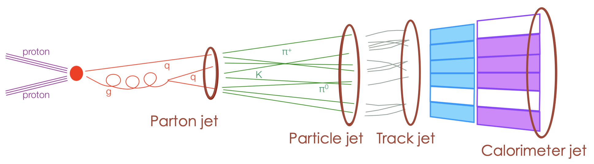
Jets are showers of collimated particles, made up mainly of hadrons, but also photons and leptons, and are the experimental signature of quarks and gluons in high energy proton-proton collisions. Due to their high production rate, jets have become a target of study to "rediscover" processes expected from the standard model, ensure that detectors behave correctly and search for new physics.

A jet is formed from the measurements of a set of neutral colored particles and its definition is not unique. In fact, the existence of a jet is dependent on the mathematical rule that defines it. These mathematical rules groups the constituents of the jet according to kinematic properties and are known as jet clustering algorithms.

Inputs

Four-vector objects are used as inputs to reconstruction algorithms, and can be:

• Stable particles defined by MC generators: particles at the MC generator level are referred to as truth particles. Jets reconstructed from these truth particles are known as "truth jets".

• Charged-particle tracks: this method uses the trajectories and momentum information of these charged particles to infer the properties of the jet. Track-based jet reconstruction is particularly useful in certain contexts as pile-up mitigation and jet tagging. The result is referred to as "track jet".

• Calorimeter energy deposits: calorimeter cells are first clustered into topological clusters (topo-clusters) using a nearest-neighbour algorithm. Calibrations are then applied to the clusters, some are: the hadron-like clusters are subject of a cell weighting procedure to compensate for the lower responce of the calorimeter to hadronic deposits, out-of-cluster (OOC) corrections for lost energy deposited in calorimeter cells outside of reconstructed clusters in the tail of hadronic shower, dead material (DM) corrections are applied on the cluster level to account for energy deposits outside of active calorimeter volumes. Jets reconstructed using only calorimeter-based energy information use the corrected EM scale topo-clusters and are referred to as EMtopo jets.

• Algorithmic combinations of tracks and energy deposits: Hadronic final-state measurements can be improved by making more complete use of the information from both the tracking and calorimeter systems. As explained in [ref1]:

  • Tracks can only be reconstructed from charged-particles hits in the inner detector, while topo-clusters are built from interactions in the calorimeters of both charged and neutral particles.
  • The angular resolution of the inner detector is much better than that of the calorimeters. Therefore tracks can be associated to the different vertices, while this is not possible for topo-clusters.
  • For low-energy charged particles, the momentum resolution of the inner detector is significantly better than the energy resolution of the calorimeters. On the contrary, at high energy, the energy resolution of the calorimeters is better than the momentum resolution of the inner detector.
  • The inner detector covers only the region |𝜂| < 2.5, while the calorimeters cover the region |𝜂| < 4.9.

  Some algorithms that use topo-clusters and tracks are Track-CaloClusters (TCC), Particle Flow (PFlow), and Unified Flow Objects (UFO).

Fig. 1: Different of the jet development.

Algorithms

As stated above, the definition of a jet depends on the mathematical rule that defines it. A clustering algorithm is expected to possess certain characteristics, as discussed in [ref2]:

• The physics interpretation of the event should not depend too sensitively on the jet definition.
• They should be independent of the design/structure of the detector.
• Minimal sensitivity to hadronisation, underlying events, and pile-up is desired, but is not always possible in practice.
• Experimentally, they should be easy to implement and (computationally) quickly executable.
• Theoretically, they need to be infrared and collinear safe to not have divergent cross-sections in perturbative calculations. Infrared safety means that the addition of a soft gluon should not change the results of the jet clustering. Collinear safety implies that splitting one parton into two collinear partons should not change the results of the jet clustering.

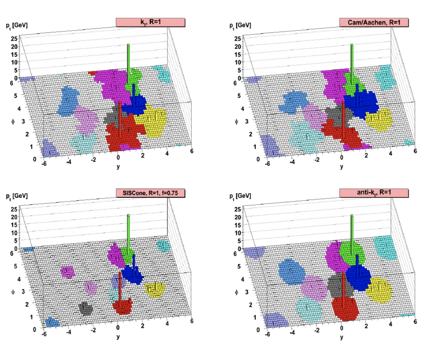
There are two main types of clustering algorithms: cone algorithms and sequential recombination algorithms.

• Cone algorithms assume that the jet lies in conic regions in $(\theta-\phi)$ space, so the jets reconstructed by these algorithms have circular edges. They are easy to implement, but are not collinearly stable. Examples of cone algorithms are: Midpoint Cone, used in Tevatron, Iterative Cone and SISCone.
• Sequential recombination algorithms assume that the components of a jet possess a small transverse momentum difference. Thus, particles are clustered in momentum space, resulting in jets with fluctuations in $(\theta-\phi)$ space.

The most commonly used recombination algorithms are $k_t$, anti-$k_t$ and Cambridge/Aachen, with anti-$k_t$ being the most widely used. It requires an external parameter, the jet radius R, which specifies up to what angle the separate partons recombine into a single jet.

Fig. 2: The four main jet reconstruction algorithms’ areas, performed on the same data with the same input radius.

Jet Energy Scale Calibration

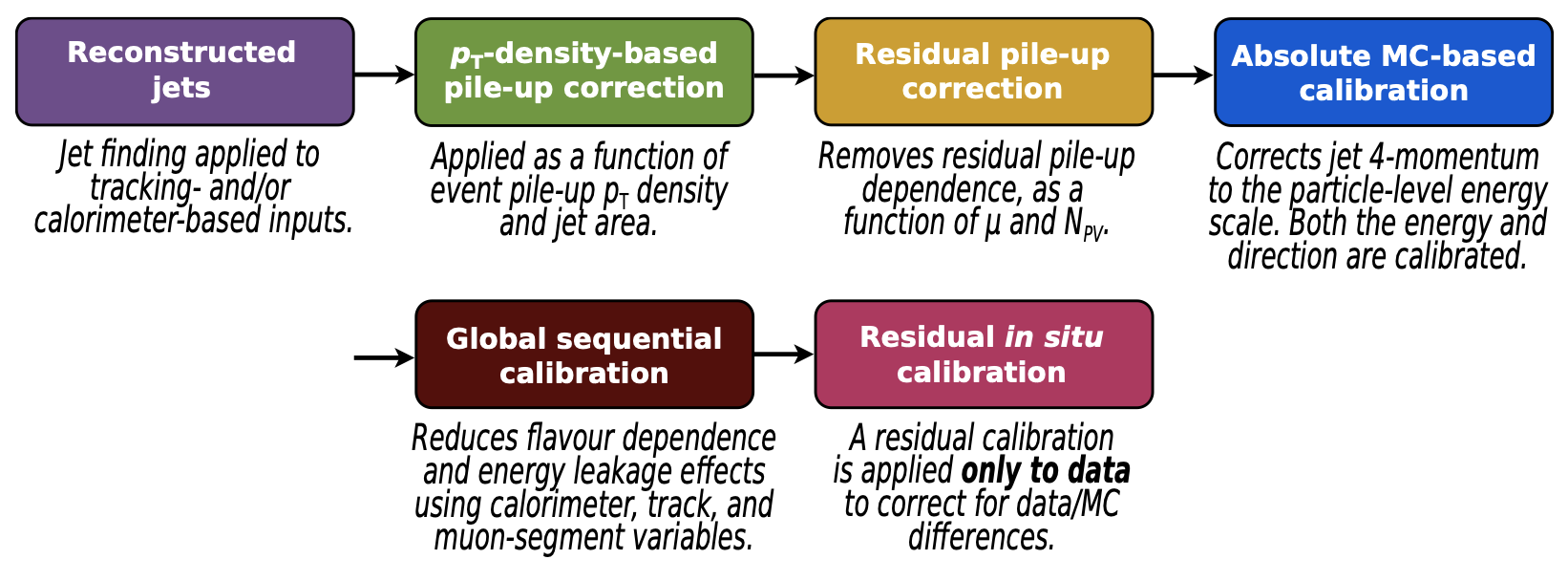
The jet energy scale calibration restores the jet energy to that of jets reconstructed at the particle level. The full chain of corrections is illustrated in Figure 2. All stages correct the four-momentum, scaling the jet transverse momentum, energy, and mass.

Fig. 3: Stages of jet energy scale calibrations. Each one is applied to the four-momentum of the jet.

The following explanations are based on New techniques for jet calibration with the ATLAS detector and Jet energy scale and resolution measured in proton–proton collisions at $\sqrt{s}$ = 13 TeV with the ATLAS detector. For further details on the specific of the methods, refer to the papers.

Pile-up Substraction

As luminosity in the LHC increases, the number of interaction during a beam crossing increases. These extra interactions are collectively referred to as “pile-up”, and its presence can have an impact on physics analyses.

Pile-up subtraction aims to remove the excess energy due to additional proton–proton interactions within the same (in-time) or nearby (out-of-time) bunch crossings. Two types of corrections are applied: one to handle the average effect of pile-up and another to fine-tune for residual effects that are not captured by the first correction.

Jet pT-Density-Based Subtraction

The extent to which a jet might be influenced by pile-up is determined by looking at two things: the 'area' (A) of the jet and the pile-up density ($\rho$) in the event.

• The 'area' of a jet is found by counting how many simulated, nearly momentum-less particles, known as 'ghost particles', are enclosed within the jet's boundaries when the particles are grouped.

• The event's pile-up density is gauged by taking the median transverse momentum per unit area, $\langle p_t/A\rangle$, from a group of pile-up 'jets' in the central region of the detector. These are not real jets but represent the organized noise from many minor collisions. This grouping is done using the anti-$k_t$ algorithm, which is good at clustering this background noise.

After determining these two factors, we correct each jet's transverse momentum to remove the pile-up effect, using the expression:

$$p^{corr}_{t} = p^{reco}_{t} - A\rho,$$

where $p^{reco}_{t}$ refers to the transverse momentum of the reconstructed jet before any pileup correction. The method assumes that the pileup is uniform across the detector and that the number of pileup jets is much larger than the number of hard scatter jets with transverse momentum above certain threshold, ensuring the median is not biased by actual collision events.

This process involves additional steps and considerations not fully detailed here. For a more comprehensive explanation, refer to the paper Pileup subtraction using jet areas.

Residual Pile-Up Corrections

The $\rho$ calculation is derived from the central regions of the calorimeter and does not fully describe the pile-up sensitivity in the forward calorimeter region. Hence, some pile-up effects remain and further corrections are needed.

The additional pile-up effect that still remains after the first correction is studied by looking at how the measured jet momentum deviates from the truth jet momentum (which we would expect in a perfect, pile-up-free world). This deviation is studied as a function of variables like $N_{PV}$ (number of primary vertices, which indicate the number of collisions) and $\mu$ (mean number of interactions per bunch crossing). These tell us about the amount of pile-up.

The final corrected jet momentum is calculated by taking the initially measured momentum and subtracting both the average pile-up and any remaining extra effects:

$$p^{corr}_{t} = p^{reco}_{t} - \rho A - \alpha(N_{VP}-1) - \beta\mu$$

$\alpha$ and $\beta$ are determined within various groupings based on the true transverse momentum of the jet that corresponds to an ideal measurement without pile-up, and the detector pseudorapidity ($\eta$), which indicates the jet's position relative to the center of the detector.

Simulation Based Calibrations

Jet energy scale and $\eta$ calibration

The jet energy scale (JES) and directional calibrations correct the mesuarements of a jet's energy and angle to reflect the true energy and direction of the particles before they interact with the detector.

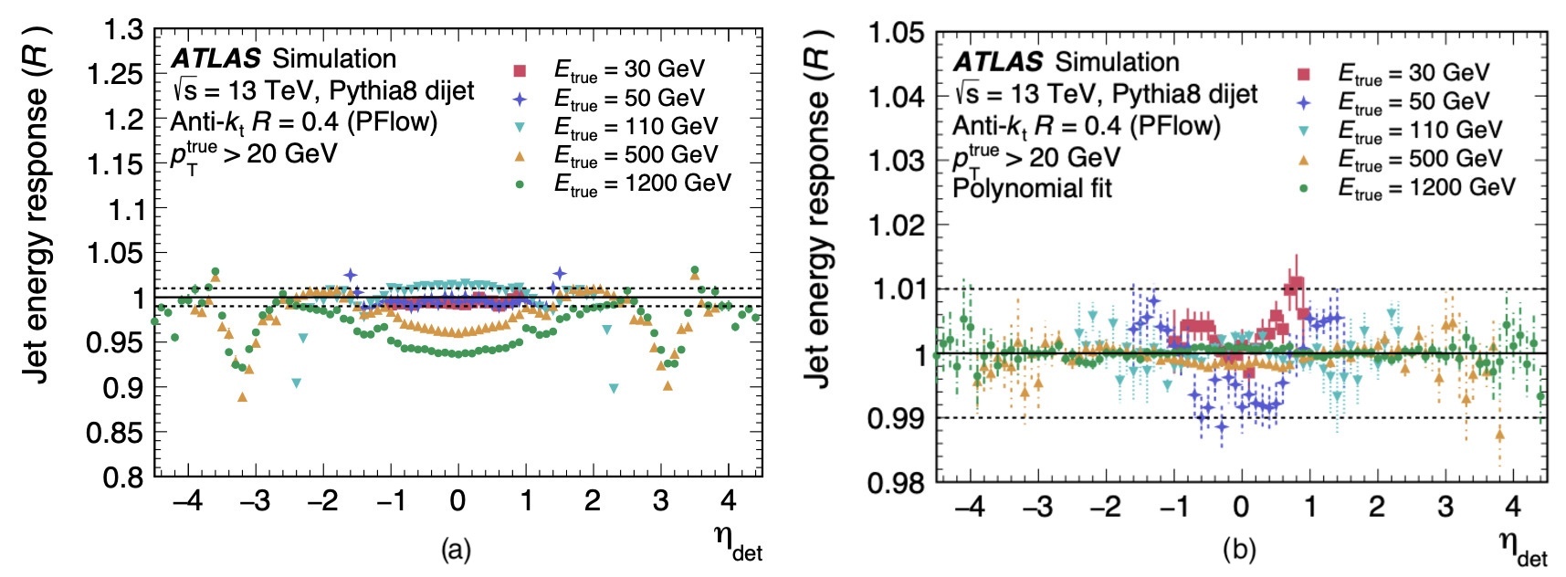
The jets measured by the detector (known as reconstructed jets) are aligned with the truth jet within a certain distance. It's required that there be no other significant jets close by to avoid confusion in the matching process. For each pair of reconstructed and truth jets the response is calculated as

$$R(E^{truth}_{jet}, \eta_{det}) = E^{reco}_{jet}/E^{truth}_{jet}$$

in bins of the truth jet energy and the pseudorapidity, where the pseudorapidity ($\eta_{det}$) is pointing from the geometric center of the detector, used to remove any ambiguity about which region of the detector is measuring the jet. The average response is parameterized as a function of $E^{reco}$ using a numerical inversion procedure.

If we plot the energy response versus $\eta_{det}$ before and after calibration (Fig. 4) we can see how the response approaches 1, i.e., how the energy of the reconstructed jets is closer to that of the true jet, which is what we aim to achieve with the calibration.

Fig. 4: Jet response at fixed energies as a function of $\eta$ (a) before calibration (b) after calibration.

There are small biases on the direction of jets after the energy correction, and an additive correction with a similar approach to the JES calibration is applied to correct them.

The global property calibration

The jet energy scale and $\eta$ calibration adjust the jet energy response based on energy and pseudorapidity. However, as explained in this reference, other factors also influence the energy response, including:

• The distribution of energy within the jet.
• The distribution of energy deposits across different calorimeter layers.
• The types of hadrons produced in the jet.

These characteristics vary depending on whether the jet originates from a quark or a gluon. Quark-initiated jets generally have fewer hadrons with a higher fraction of the jet's $p_T$, leading to deeper calorimeter contributions. In contrast, gluon-initiated jets typically contain more hadrons with lower $p_T$, resulting in a lower calorimeter response and a broader transverse profile.

The jet $p_T$ response is also affected by the Monte Carlo (MC) model. While most MC predictions show similar behavior for quark-initiated jets, the differences for gluon-initiated jets can be significant.

To reduce jet-to-jet response variations, the global property calibration is employed, using two methods: global sequential calibration (GSC) and global neural network calibration (GNNC).

Global Sequential Calibration (GSC) applies a series of multiplicative corrections to account for differences in calorimeter responses to different types of jets, improving jet resolution without altering the jet energy response. It relies on global jet observables such as:

• The longitudinal profile of energy deposits in the calorimeters.
• Tracking information matched to the jet.
• Activity in the muon chambers behind the jet.

Each correction to the jet four-momentum is derived and applied independently and sequentially. However, GSC is constrained to using relatively uncorrelated variables for correction. Using correlated variables would cause each sequential step to interfere with previous corrections.

The Global Neural Network Calibration (GNNC) addresses the limitations of GSC. A deep neural network (DNN) is trained to perform a simultaneous correction using a wide variety of jet properties. This allows the use of correlated variables for determining the global jet property correction. Unlike GSC, the DNN is designed to correct the jet $p_T$ response, which is crucial for analyses based on jet $p_T$.

Both calibration methods have a small overall impact but significantly improve the calibrations for different classes of jets, enhancing energy resolution. Additionally, these calibrations reduce differences between MC predictions for the jet energy scale, leading to smaller modeling uncertainties.

In-situ Analysis

All the steps previously explained aim to correct jets on the particle level to get simulated and data jets closer to having the truth energy and mass. Now, we want to account for the differences between data an simulation. This differences are caused by imperfections in simulation of the detector material or the involved physics processes. In this calibration we calibrate data to match the simulation, given that the MC based calibrations calibrated the simulation to match the true energy scale, which is the scale in which we would like to have the data.

Fig. 5: The in-situ jet energy scale calibration process.

The in situ calibration provides validation of the previos MC calibration of jets by comparing the data-to-MC difference between the $p_T$ balance of a jet against a well-calibrated object or system. For this, the jet response is as the average ratio of the jet $p_T$ to the reference object $p_T$:

$$R_{\text{\it{in situ}}} = \Biggl\langle\frac{p_T^{jet}}{p_T^{ref}}\Biggr\rangle ,$$

where the reference objects are $Z(\rightarrow\mu\mu)$, $Z(\rightarrow ee)$ or $\gamma$. However, $R_{\text{\it{in situ}}}$ is sensitive to effects such as the presence of additional radiative jets or the transition of energy into or out of the jet cone. A double ratio, insensitive to these secondary effects provided they are well-modelled in simulations, is defined:

$$C = \frac{R_{\text{\it{in situ}}}^{data}}{R_{\text{\it{in situ}}}^{MC}}$$

The calibration factor to the jet four-momentum can be obtained by a numerical inversion of this doubleratio as a function of jet $p_T$ , and as a function of $\eta_{\text{det}}$ in $\eta$-intercalibration.

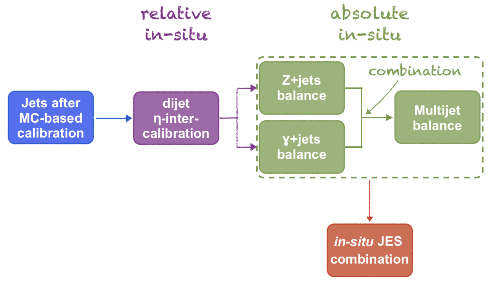
In in-situ analysis, there are two sequential steps: relative in-situ calibration (or $\eta$-intercalibration) and absolute calibration.

The relative in-situ calibration aligns the energy scale of forward jets ($0.8 < |\eta_{det}| < 4.5$) with the energy scale of central jets ($|\eta_{det}| < 0.8$). This alignment is achieved using the transverse momentum ($p_T$) balance in a dijet system, where forward jets are generally better understood. The calibration involves calibrating all regions relative to each other by solving a set of linear equations, a process known as the matrix method.

The absolute calibration adjusts the absolute jet energy scale in data to match the scale in simulation. This is done by exploiting the $p_T$ balance between the hadronic recoil and a well-calibrated reference object, such as a $Z$ boson or a photon. The following methods are aimed to achieve this:

1. Direct Balance (DB): This method balances the $p_T$ directly between the reference object and the jet.
2. Missing Projection Fraction (MPF): This method balances the $p_T$ between the reference object and the entire hadronic recoil of the detector. The MPF method is the most commonly used.
3. Multi-Jet Balance (MJB): For higher $p_T$ jets, this method uses already calibrated lower-$p_T$ jets as reference objects to balance with the higher $p_T$ jets.

The results from different absolute in-situ calibrations are then statistically combined to achieve a final calibration.

More Information

For further details on the specific of the introduced methods, refer to the papers New techniques for jet calibration with the ATLAS detector and Jet energy scale and resolution measured in proton–proton collisions at $\sqrt{s}$ = 13 TeV with the ATLAS detector.