PyROOT framework
The framework utilizes the Python language and interfaces with ROOT.
Get the code
Access the code and documentation via the button below:
The framework consists of two main parts:
- the analysis part, located within the "Analysis" directory: it performs the particular object selection and stores the output histograms;
- the plotting part, located within the "Plotting" directory: it makes the final Data / Prediction plots.

Read about this analysis in the Example Analyses with the 13 TeV Data for Education section
Get the data
The 13 TeV ATLAS Open Data are hosted on the CERN Open Data portal and ATLAS Open Data portal in this documentation. The framework can access the samples in two ways:
- reading them online directly (by default, they are stored in an online repository);
- reading them form a local storage (the samples need to be downloaded locally).
First time set up
The only requirement is having Python installed:
- Python 3: The master branch of the framework uses Python 3. Ensure you have it installed.
- Python 2: A separate branch for Python 2 is available if needed.
Refer to the official Python installation guide for more details on getting Python set up on your machine.
Running an Analysis
The analysis code is located in the Analysis folder, with files corresponding to the examples of physics analysis documented in Physics analysis examples. The naming of the analysis files follows a simple rule: "NNAnalysis", where NN can be HZZ for example.

The files in the root directory of the installation are the various run scripts. Configuration files can be found in the Configurations folder.
As a first test to check whether everything works fine you can simply run a preconfigured analyis via
python3 RunScript.py -s "Zmumu"
What you have done here is to run the code in single core mode and specifying that you only want to analyse the Zmumu sample as defined in the Configurations/HZZConfiguration.py. The runscript has several options which may be displayed by typing
python3 RunScript.py --help
The options include:
-a,            --analysis              overrides the analysis that is stated in the configuration file
-s,            --samples               comma separated string that contains the keys for a subset of processes to run over
-p,            --parallel              enables running in parallel (default is single core use)
-n NWORKERS,   --nWorkers NWORKERS     specifies the number of workers if multi core usage is desired (default is 4)
-c CONFIGFILE, --configfile CONFIGFILE specifies the config file to be read (default is Configurations/Configuration.py)
-o OUTPUTDIR,  --output OUTPUDIR       specifies the output directory you would like to use instead of the one in the configuration file
The XConfiguration.py files specify how an analysis should behave. The Job portion of the configuration looks like this:
Job = {
    "Batch"           : True,              #(switches progress bar on and off, forced to be off when running in parallel mode)
    "Analysis"        : "HZZAnalysis",     #(names the analysis to be executed)
    "Fraction"        : 1,                 #(determines the fraction of events per file to be analysed)
    "MaxEvents"       : 1234567890,        #(determines the maximum number of events per file to be analysed)
    "OutputDirectory" : "resultsHZZ/"      #(specifies the directory where the output root files should be saved)
}
The second portion of the configuration file specifies the locations of the individual files that are to be used for the different processes can be set as such:
Processes = {
    # H - ZZ - 4lep processes
    "ggH125_ZZ4lep"         : "https://atlas-opendata.web.cern.ch/atlas-opendata/samples/2020/4lep/MC/mc_345060.ggH125_ZZ4lep.4lep.root", #(single file)
    ...
}
The names chosen for the processes are important as they are the keys that are used later in the infofile.py to determine the necessary scaling factors for correct plotting.
Now we want to run over the full set of available samples. For this simply type:
python3 RunScript.py
Use the options -p and -n if you have a multi core system and want to use multiple cores. Execution times are ~ 40 minutes in single core mode or ~ 25 minutes in multi core mode with 4 nodes.
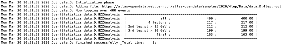
If everything was successful, the code will create in the results directory (resultsNN) a new file with the name of the corresponding sample (data_A, ttbar_lep,...).
Plotting the Results
The plotting code is located in the Plotting folder and contains the following files:
- Histogram manipulation (Database.py): The functionality found here implements a metadata database used to manipulate the histograms;
- Plot variaties (Depiction.py): Depictions define certain standardized plot varieties;
- Paintable definitions (Paintable.py): splits the problem of plotting something into logical pieces;
- Plot style (PlotStyle.py): The general style that is to be applied is defined here;
- infofile (infofile.py): MC sample name, DSID, number of events, reduction efficiency, sum of weights and cross-section.

Results may be plotted via:
python3 PlotResults.py Configuration/PlotConf_AnalysisName.py
In our example case the name of the analysis is HZZAnalysis, so type:
python3 PlotResults.py Configuration/PlotConf_HZZAnalysis.py
The resulting histograms will be put into the Output directory.
The plotting configuration file enables the user to steer the plotting process. Each analysis has its own plotting configuration file to accomodate changes in background composition or histograms that the user may want to plot.
General information for plotting include the Luminosity and InputDirectory located at the top of the file:
config = {
    "Luminosity"     : 10064,
    "InputDirectory" : "resultsHZZ",
    ...
The names of the histograms to be drawn can be specified like so:
"Histograms" : {
...
    "invMassZ1"       : {"rebin" : 3},
    "invMassZ2"       : {"rebin" : 3},
"lep_n"           : {"y_margin" : 0.4},
...
Note that it is possible to supply additional information via a dictionary like structure to further detail the per histogram options. Currently available options are:
rebin    : int   - used to merge X bins into one. Useful in low statistics situations
log_y    : bool  - if True is set as the bool the main depiction will be drawn in logarithmic scale
y_margin : float - sets the fraction of whitespace above the largest contribution in the plot. Default value is 0.1.
Definition of Paintables and Depictions
Each Plot consists of several depictions of paintables. A depiction is a certain standard type of visualising information. Availabe depictions include simple plots, ratios and agreement plots. A paintable is a histogram or stack with added information such as colors and which processes contribute to said histogram. A simple definition of paintables may look like this:
'Paintables': {
    "Stack": {
        "Order"     : ["Other","ZZ","HZZ"],
        "Processes" : {
            "HZZ" : {
                "Color"         : "#ff0000",
                "Contributions" : ["ggH125_ZZ4lep","VBFH125_ZZ4lep","WH125_ZZ4lep","ZH125_ZZ4lep"]},
            ...
    },

    'Higgs': {
        'Color': '#0000ff',
        'Contributions': ['ggH125_WW2lep']},

    "data" : {
        "Contributions": ["data_A", "data_B", "data_C", "data_D"]}
Stack and data are specialised names for paintables. This ensures that only one stack and one data representation are present in the visual results. A Stack shows the different processes specified in "order" stacked upon each other to give an idea of the composition of the simulated data. The definitions for these individual processes are defined under "Processes". Each process has a certain colour and a list of contributing parts that comprise it. These contributing parts have to fit the keys used in both the run configuration and the infofile.py.
data is a specialised paintable which is geared toward the standard representation of data. Since the data does not need to be scaled there is no need to align the used names in contributions with those found in the infofile.py. However, they still have to fit the ones used in the configuration.py.
All otherwise named paintables (like "Higgs" in the example) are considered as "overlays". Overlays are used to show possible signals or to compare shapes between multiple overlays (for instance in a HWWAnalysis).
The paintables can be used in depictions like so:
"Depictions": {
    "Order"       : ["Main", "Data/MC", "S/B"],
    "Definitions" : {
        "Data/MC": {
            "type"       : "Agreement",
            "Paintables" : ["data", "Stack"]},

        "Main": {
            "type"      : "Main",
            "Paintables": ["Stack", "data"]},

        'S/B': {
            'type'       : 'Ratio',
            'Paintables' : ['Higgs', 'Stack']},
    }
There are currently three types of depictions available: Main, Agreement and Ratio. Main type plots will simply show the paintables in a simple plot fashion. Ratio type plots will show the ratio of the first paintable w.r.t. the second paintable. Agreement type plots are typically used to evaluate the agreement between two paintables (usually the stack of predictions and the data).
The order of the depictions is determined in line 2 of the code example above.
If everything was successful, the code will create in the output directory (Output) the corresponding plots defined in Configurations/PlotConf_AnalysisName.py.

In Depth Information
Analysis Code
The analysis code is located in the Analysis folder. It will be used to write out histograms for the individual input files which will be used for plotting purposes later.
The basic code implementing the protocol to read the files and how the objects can be read is in TupleReader.py. Have a look there to see which information is available. The general analysis flow can be found in Job.py whereas the base class for all concrete analyses is located in Analysis.py.
It is recommended to start out by modifying one of the existing analyses, e.g. the HZZAnalysis located in HZZAnalysis.py. If you want to add an analysis, make sure that the filename is the same as the class name, otherwise the code will not work.